Personal (Agent) Preference, Systems Constraints and The Games We can Play

I was in a resort last week end. There was a trampoline (only that!) and all the kids were getting attracted to get on to it. However, soon the kids realized that the trampoline could not take all of them jumping. Then one girl came up with a game. She made all the kids sit in a circle on the circumference of trampoline and one by one would go to the centre and jump. Rest of them would feel the vibrations (?) and enjoy. We were pleasantly surprised by this game and initiative by a 8-9 year old.

Next day, the same trampoline was occupied by another group of kids. Initially they also had the same chaos, confusion and even fight about them jumping. But, surprisingly, this group also ended up going one by one in their turn and jump in middle. Only thing they changed is, they slept along the circumference rather than sitting. Another difference was, the previous day kids went it order of their age, where and the kids on second day created some random order.

While the kids were resolving their issue on second day, I also found different groups of people playing different games in the very large lawn area (some one and half acres). Some were playing badminton, some football, and some cricket. I just started wondering what is that which is making the kids on trampoline play almost similar games every time, while the people in lawn get to choose different games.

Looks like there are two predominant parameters playing their role in deciding the types of game we can play in a a system (trampoline or lawn). One is the personal (agent) preference(s) and the other is system constraint(s). In case of trampoline, the system constraints were very rigid. The kids had limited space, the weight it could bear was limited. Hence, even when every one had their own preferred game to play on it, they ended up playing a game which accommodates the system constraints (and a part of their preferences as well).

In case of lawn, the the system constrains are bit more relaxed (in terms of weight it can hold, space it provides, and so on). Hence, the system allows the agents to reveal and realize their preferences more liberally. But still, one has to understand that there are constrains here as well. For example, one can not play fly a plane over there or do archery (as it can hurt the other groups using the same space). However, Note that not always the size of the space determines the system constraints. For example, a set of cards can give us more possibility than a lawn!

The constraints of the system can be divided into three types. The first one is obligated things. They are the properties which are mandatory to be considered when we work in the given system. For example, in trampoline, it is obligated that people play together (according to currant societal norm).  Then come the permitted ones, which are optional. Finally, there are some things which are permitted. The total weight of the kids on trampoline should not cross 140kgs. All the three system constrains influence the games we can play in the environment. We can not play any game, which has any forbidding constraint. That violates the system (like having kids which together weigh more than 140kgs on trampoline). Not following the obligated constraints also has the similar implication. Hence, the choice for the actors remains only in the area of  permitted acts. When this choice no more exists (meaning – no permitted acts are there) or there is very limited choice (very few permitted acts), then the actors end up playing the stricter games which are just governed by obligations and forbidden acts. Here, the personal preference plays no role (for no choice) or very limited role (for very few permitted acts).

When there are larger choices in the system, then number of games we can play also increases. Assume that if there are n permitted acts. Then we may have 2^n combinations of the choices can be clubbed with the obligations and forbidden acts. Hence, we can create games using some many parameters! Here, the personal preferences can be used to choose the permitted parameters and design games. Hence, we are more free in this system to create our games.

It looks like, in any space, the system constraints augmented with individual preferences determine the games played in the space. If there are more permitted acts in the system, the agents tend to be more free to decide the games they want to play.

(I would like to thank Prof. Srinath for introducing different types of constraints).

Semantics as a Whole: Perceptive and Cognitive Semantics

Conventionally, in the literature, there are three types of “meanings” — Pragmatic meaning, Semantic meaning and Conceptual meaning. The term “semantics” is related to the “semantic meaning”. Wikipedia gives the following definition:

“Semantic is the study of meaning. It focuses on the relation between signifiers, like words, phrases, signs, and symbols, and what they stand for; their denotation. Linguistic semantics is the study of meaning that is used for understanding human expression through language. Other forms of semantics include the semantics of programming languages, formal logics, and semiotics. In international scientific vocabulary semantics is also called semasiology.”

Many other definitions of semantics also essentially define it as “study of meaning”. However, this definition of has been used in very loose sense and hence the area of semantic mining from the given data does not seem to have a concrete boundary. Because of that, most of the work in current day semantics mining focuses on a shallow semantics.

We, in WSL (Web Sciences Lab) at IIITB are working on identifying the classes of semantics mining problems. We claim that there are two types of semantics namely “perceptive semantics”  and “cognitive semantics”.

Consider the following pictures.

1. A bus accident

2. Children on picnic

3. School children picnic

The perceptive semantics would tell that images (1) and (3) are similar as both have bus and people. It just identifies the features. However, the cognitive semantics tells that the images (2) and (3) are similar as both of them are describing picnics.

Perceptive semantics mining focuses on the features and their relations. For example, in text a perceptive semantics method might identify that car and fuel are co-related. However, it dos not go beyond it. Another example may be the following image.

The image shows that there is some function where two donkeys and some people are part of. This is a  perceptual understanding (perceptual semantics).

The cognitive semantics mining for the same picture tells that it is a function of donkeys’ wedding and it means that “it has not rained in that area this year and people might be in trouble”. Thus, while perceptive semantics tells that there are donkeys and people by answering the question of “what are they”, cognitive semantics tells “why are they here?”.

It has been observed that in linguistic literature, there has been a similar classification  — semantics and pragmatics. However, when we look at the semantics as a notion across domains, we claim that our classification makes sense.  We claim that both semantics and pragmatics, mentioned in the linguistics literature are different levels of semantics. Hence, rather than looking at them separately, we should identify the factor which makes the difference. The perceptive semantics (which is similar to linguistic semantics) is the semantics between constructs of a domain due to the perceptive activity of our brain. However, the cognitive semantics (linguistic pragmatics)  give contextual information and inferences between the given concepts of the domain and it is due to our cognitive abilities and the memory.  Hence, looking at the semantics as continuous space where there are two fuzzy classes — perceptive semantics and cognitive semantics make more sense.

When it comes to mining semantics from given user generated data (any kind of data – image, video, text , …), we should clearly understand what type of semantics we are looking at. If we are looking for description of data (without any contextual inference), then perceptive semantics mining is the way to go. For example, if we want to identify the all images where bus and children are coming together, then we treat it as perceptive semantics problem. However, if we are looking for contextual inference augmented with cognitive insights, then we have to perform  cognitive semantics mining. Most of our current day problems involving decision support look forward for cognitive semantic mining approaches. Let it be identification of a journal article for a doctor related to a patient or be it identification of a resolver for a given insurance claim, we look for contextual inference.

Value of a Network: Different Perspectives and Observations

Many times, a new person joining a network (social or financial) has an impact on the members already part of the network. This kind of impacts contribute to the increase or decrease in the value of the network. These impacts in turn decides the growth or decay of the network. In this paper, we will look into some examples of such networks in current time. We will discuss many different perspectives of the network value and many laws proposed to quantify them. There have been many questions raised on the validity of these laws. hence, we will look into the issue of validity of these laws. At the end, we will discuss the different interpretation of these laws and try to put them in right perspective.

1. Introduction

When we buy some goods/service or get into a social community, we will implicitly become a part of a network. For example, buying a set-top-box(STB) connection make you a part of all the consumers having the same set-top-box connection. Even though the structure of the network and the properties of the elements (here people) is not clearly known, the group is assumed to be connected due to the common service/good or relation. The growth of such network many times depends on the value of the network when new members join them. We will look into some of the known networks and try to observe the special behavior of the networks as they grow.

Maruti Cars: Maruti is an Indian car manufacturing company. It was founded in 1981. At the time Hindustan Motors, Fiat (as Premier Automobiles Limited) like companies were present in Indian car market and selling cars. But, Maruti started becoming popular day by day. As more and more people bought Maruti cars, more and more service stations were started. These were not always started by Maruti, but sometimes were just authorized by them. As the number of Maruti cars increased, it created the opportunity to establish new service stations (due to more number of cars) and also made spares cheap due to mass production. As more number of service stations were available and spares became cheaper, people inclined towards buying more Maruti cars. Hence, whenever a person buys a Maruti car, he gets the value for the money he has as the car. But, he will also get a complementary benefit of cheap and highly accessible service. This benefit is shared between all the Maruti car owners. Hence,

Buying a Maruti Car = A Car Worth the Money Spent + Cheaper Spares + Accessible Service

The Cheaper Spares + Accessible Service part contributors to gain for all the Maruti car owners. According to the statistics of March-2011, Maruti holds 48.74% of the Indian car market share!

Migration of People to USA: America was discovered in 1492. Then it was a land of indigenous tribes. Hence, initially life was very difficult for the people coming and settling over there. As the number of adventurous and visionary people started coming to USA, the life started getting better. At some point of time, it started becoming an attraction for people looking for greater opportunities. So, people with skills to exploit the opportunities started moving to America. Due to the skilled people, there began a faster development and created more opportunities. Thus, as the number of skilled people entering USA increased, the value of the USA as a society increased. It can be given as,

New Skilled Person Entering USA = The Person Getting Opportunities Worth the Value Spent to Enter + More Opportunities + Better Lifestyle

The More Opportunities + Better Lifestyle will be the gain for all the Americans due to one person. We observe that one person entering USA increases the value of the society in USA.

Road Networks in City (More Vehicles on the Road): Assume there is a road network in a city which has no vehicles. When the first vehicle starts using it, it will have no problems like overtaking, honking, traffic jam, accidents, parking etc. But, as the number of vehicles using the same road network increases, the earlier drivers start feeling it more problematic. They will start facing all the problems mentioned above. Even the travel time increases. The cost of travel also increases due to slow driving. In other terms, whenever a new car joins the same road network, even though car owner gets the comfort of traveling a new car, he decreases the speed at which the traffic moves in the city (increases the the travel time). He also increases the cost of the travel due to the slow drive. We can represent it as,

New Vehicle Joining the City Traffic = Comfort Worth the Value of the Car to Owner + Slower Traffic + More Travel Cost

Slower Traffic + More Travel Cost is the reduction in the overall traffic system due to increase in the number of vehicles on the road.

From all the examples above, we can observe a very dominant behavior of the networks. When a new elements(person, car etc.,) is added to the network, the elements adds extra benefit or cost to all the other elements of the network. So, generically we can express this as,

New Element Joining the Network = Value Equal to Expenditure Made to Join Network + Some Benefit/Cost to all the Members of the Network

There are many such example around us which show this kind of behavior. The following are the

• People forming villages.
• People buying more Nokia phone in early 2000s.
• People buying Hero Honda vehicles in mid 90s.
• Internet.
• Arrival of IT Companies in Bangalore.
• Plantations.
• Electricity Consumption.
• Mobile Network Congestion.

In the examples seen, we have to observe that, when a new member enters a network, the network might get benefited in some aspects and might incur cost in some other aspects. So, whenever a new member joins the network, we have to look into all the aspects and take the aggregated value add to understand whether the network is getting benefited or incurring cost as a whole. If the aggregated value add is positive, network made benefit and when the aggregated value add is negative, network incurred cost.

If the network gets benefited , in aggregate, from the addition of new member, then there will be higher motivation for the people inside the network to welcome more people and also there will be higher motivation for new members to join. However, if there is absolute cost incurred by the network members and the new member when the new member joins the network, then there will be negative motivation for non members to joining the network.

2. Value of a Network

The aggregated value add is the way in which a network gets its overall value. When a new member enters the network, in case of existence of benefit, the value of the network increases and in case if the cost is incurred, the value of the network decreases. This growth of value of the network indicates a lot of future trends. Hence, many people have tried to quantify the value of the network in different aspects. The following are few interesting laws trying to quantify the value of the network.

a) Metcalfe’s Law
Robert Metcalfe is the co-inventor of Ethernet. He wanted to explain people why they should buy more and more Ethernet card. Hence, he proposed a law which asserted that the value of the Ethernet network is proportional to the square of the number of Ethernet cards connect in it. Hence, though the cost of adding new element to the network increases linearly, the value of the network due to the addition of new element increases quadratically.

The intuition for value of the network is derived from the possible number of connections in the network. If we consider a directed network with n nodes, then the maximum number of connection possible in that network is n(n-1) (if we do not consider the self loops). This is in the order of n². Hence, it is looks intuitive that the value of the network increases quadratically. Figure 2 gives more insight about the claims of Metcalfe’s law (the image taken from wikipedia).

Example to explain the intuition behind the network value claims by Metcalfe’s law. The value of the network here is the “maximum number of connection possible”.

This makes network gain more value due to the addition new network element. This looks beneficial to grow the network because, for such a growth, there will always be an n, for which:

1. The value of network becomes greater than cost, and
2.   For any value greater than n, value of network increases faster than the cost incurred, and cost starts becoming negligible.
3. The network starts increasing its value in almost quadratic terms.

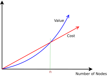
The diagrammatic representation to show that the quadratic value will always cross the linear value for some value “n”. Then the linear value starts becoming negligible.

The above figure shows this phenomenon in a graph. We can observe that once the number of elements in the network crosses  n, the value of the networks becomes positive (even if it is negative earlier due to the cost of adding new nodes). After this stage, as the network grows, the linearly growing overall cost starts becoming negligible compared to the quadratically growing value of the network.

The law was later formalized by George Gilder for all the networks in 1993. He claimed that this law is not only applicable to the device networks (like Ethernet), but is also applicable to networks with users in it (economic network, business network etc).

b) Reed’s 3rd Law
Metcalfe’s law became famous due to its intuitive quantification of the value of the network. In 2001, David P. Reed, an American computer scientist came up with a new law called Reed’s Law for quantifying the value of a network. He said that the Metcalfe’s law underestimates the value of the network. He claimed that the law is highly applicable for large scale networks like social networks (more on Reed’s law at: http://en.wikipedia.org/wiki/David_P._Reed, http://en.wikipedia.org/wiki/Reed’s_law). The statement of Reed’s Law goes as follows:

As networks grow, value shifts: Content (whose value is proportional to size) yields to Transactions (whose value is proportional to the square of size), and eventually Affiliation (whose value is exponential in size)

In Reed’s law,

• The meaning of the term content is the number of nodes.
• The meaning of the term affiliation is the social and business relationship.

Reed’s law tells that when a network starts building, it will have value only because of its individual members, as there are not transactions between members and no affiliations too. But, later, the members of the network get into transactions. Because of the transactions, the value of the network becomes quadratic in nature(similar to Metcalfe’s Law). Due to the transactions, the members will come together and form different communities. The real value of the network becomes exponential due to formation of such of communities.

The intuitive proof of Reed’s Law goes like this. When members start transacting, in a n member network, the maximum number of transaction each person can do is n-1. Hence, the total number of transactions in the network will be n x (n-1), which is O(n²). Hence, Reed claims that the value of the network due to transactions is quadratic.

When the member start forming the communities, the maximum number of Group-Forming-Networks(GFC) people can form with other members is 2ⁿ – n – 1. A GFN is nothing but any community formed by the some members of the network. 2ⁿ is the cardinality of the power set of n members. We subtract n from with a naive assumption that there can not be single member communities. We subtract 1, as it represents the number of empty sets in the power set. 2ⁿ – n – 1 is in the order of O(2ⁿ). Hence, Reed claims that the value of the network due to the affiliations is exponential in nature.

c) Beckstrom’s Law
Beckstrom’s law was proposed by Rod Beckstrom in 2009. Beckstrom claims that this law can be used to evaluate any kind of network including electronic networks, social networks, supports networks and Internet. The laws states that:

The value of a network equals the net value added to each user’s transactions conducted through that network, summed over all users.

The Beckstrom’s law takes completely different look at the value getting added to the network. Instead of looking into structure and number of nodes as the input for calculating the value of the network, Beckstrom’s law looks at each transaction happening in the network (represented as an edge) as the input for calculating the value of the network. The law looks at the factor of “how valuable is the network for each user“. This is calculated by aggregating all the benefits a member gets due to the presence of the member in the network. This factor in aggregation over all the members is used to calculate the value of the complete network.

It is not that each transaction in the network adds value to the member. It is possible that due to presence of the network, the member might incur more cost. This cost is also taken care when the value of the transactions is calculated. Hence, if the member is incurring cost due to the presence of the network, the value of the network might reduce. This is a new way of looking at the value of network, which was not done by both Metcalfe’s law and Reed’s law.

To understand how value is derived from the network, let us look at an example. Assume that you wanted to buy an laptop. You visit the stores near by and understand that the minimum prize it is available for is Rs. 30000 and you decide to buy. Now, while browsing, you come across the same model of the laptop for Rs. 28000 on Flipkart. You also get to know that, they provide additional 3-years warranty free complimentary (which is worth Rs. 2000). Now, we know that by buy on-line, we will save Rs. 4000 in total. This is the value generated by us by the transaction. Similarly, the Flipkart will also gain in the transaction, say Rs.1000. Similarly, there might be many nodes in the network which will get value add. The value of the network will be the aggregate (sum) of all the gains.

Beckstrom’s law takes care of the temporal aspect of the network value. When a transaction adds value to the network, its value will not remain the same over time. As the time progresses, its values starts decaying. Hence, after some time, if there no transaction in the network then the network starts losing the value as time passes.

3. Review and Interpretation of Laws

Questioning the Validity of Metcalfe’s Law (Metcalfe’s Law is Wrong): There has been many criticism on the Metcalfe’s and Reed’s Laws. The first argument focuses on the the number of connections handled by each node in the network. The argument says that the Metcalfe’s and Reed’s Law can not be applied to quantify the value of networks involving people as the members. People have limit to the number of stable connections they can manage. Once the number of connections get saturated, the person can not get involved in any more connections. So, growth rate is not always quadratic and is restricted by the saturation of connection handling capability of people.

The other kind of argument talks about the nature of connection distribution in network. The claim is “the value of the network with  n member is of the order of n log(n)”. The basis for the claim lies in the assumption that the distribution of connections follows the Zipf’s law. Hence, the connection distribution for each member for all other members looks like 1, ¹⁄₂ , ¹⁄₃ , … , ¹⁄_n-1. It mean that if there is observation on the connection time of a member with other members, and if the maximum connection time is normalized to 1, then other connection times will look like 1, ¹⁄₂, ¹⁄₃, … , ¹⁄_n-1. So the value of the network contributed by one member is 1 + ¹⁄₂ + ¹⁄₃ + … + ¹⁄_n-1.For infinitely big network this series converges to log(n). As there are n such member, the value of the network is n log(n).

Interpretations and Analysis of the Laws: As we saw these laws, and their criticisms, it was getting more and more evident that we are misunderstanding the laws in some conditions. We have intuitively understood that even though all these laws talk about the {value of the network}, the value is measured in different contexts for each of the laws. Hence, in this section, we will try to understand different context where these laws will be used and their different interpretations.

Interpretations of Metcalfe’s Law: Metcalfe’s law is used in the context, where we need to understand the value of the network in terms of number of connection. Here are some the observations.

1. Metcalfe’s Law values the network in terms of the number of possible connections in the network. The number of possible connection is also an indication of number of possible transactions. Note that it is the upper bound of the network value. Hence, we should not misunderstand the the value of the network will always be at its maximum.
2. Metcalfe’s Law is highly applicable to small network like LAN, where almost every machine is connected to every other machine. In such small networks, it may be possible that the maximum value is reached by such network.
3. The law has the limitation when we try to apply this on network with people as the members. This is due to the saturation of the number of connections an individual member can handle. The law ignores the fact of probability of the connection between different members and hence ends up misleading for larger networks.

Interpretations of Reed’s Law: Reed’s law used in the context of understanding society value in the network. We interpret Reed’s law as below.

1. Reed’s law talks about the value of the network being proportional to the exponent (2ⁿ) of the number of member. This means that, the value of the network found using the Reed’s law is the value in terms of the number of different groups that can be formed in the network.
2.  The value of the network formed puts an upper bound on the actual value of the network. Even if the the value of the network may not be equal to the value proposed by Reed’s law, it can never cross it. Hence, Reed’s law defines the boundaries of the value of the network in its own context.
3. The Reed’s law is applicable in the small networks which show the tendency of heterogeneous group formations. For example, in the a small apartment society, there will be different groups like sports club, music club, drama club, trekkers etc.,. There, the value of the network might be very near to the value proposed by Reed’s law. But, when the network size increases, then value of the network will not grow exponentially. The law ignores the fact of probability of the connection between different members and hence ends up missing this point.

Interpretations of Beckstrom’s Law: Beckstrom’s Law talks about the value of a network due to the transactions in the network.

1.  The law rightly identifies the transactions between the members as the potential contributors to the network value.
2. The law has a provision for network value to decay due to the increased cost in transactions. This makes sure that many other factors causing negative effect on the value of the networks are also considered.
3.   The decay of the generated value over time tells that value of the network is temporal in nature. This is a new way of looking at the value of a network. Due to the temporal nature, the value of network starts decreasing when the number of transactions in the network stop. There will be threshold value of transaction value. If this transactions do not generate this threshold value, then the value of the network starts decreasing.
4. This can not capture the value added only by the presence of a member in the network. For example, presence of a film start in a commercial good network might bring many other fans to the network. These fans may in turn add value to the network. But, the law does not work in that context.

We have to understand the contexts of the applicability of the laws to understand them better. Like Moor’s law, these laws are not immutable laws as well. They are laws which indicate tendencies but are not strict in nature.

4. Conclusion

It has been observed that many networks increase or decrease in their value due to the addition of new members. This phenomena can in turn be the reason for the growth or decay of a network. Due to this kind of importance, there have been many attempts to quantify the value of a network by many people. Metcalfe, Reed and Beckstrom came up with own laws to quantify the value of a network. They looked into different aspects of the networks and tried to quantify the value of the networks in those contexts. But, it has always been misunderstood that all of them proposed the value of for a network in the same context. Metcalfe and Reed have ignored some important factors like saturation of limit of connections for individual human beings while proposing the laws. These has become a reason for lot of controversies and criticisms. But, when we keep the contexts in the view, then these laws give us lot of important properties.

REFERENCES

1. Hendlera, J and Golbeck, J. Metcalfe’s Law, Web 2.0, and the Semantic Web. Web Semantics: Science, Services and Agents on the World Wide Web.
2. Reed, D.P. The Law of the Pack. Harvard Business Review. 2001
3. Odlyzko, A. and Tilly, B. A refutation of Metcalfe’s Law and a better estimate for the value of networks and network interconnections. Manuscript, March. 2005
4. Briscoe, B. Odlyzko, A. and Tilly, Metcalfe’s Law is Wrong. IEEE Spectrum. July 2006
5. Beckstrom, R. A New Model for Network Valuation. 2009

Is ln(2) = (1/2)ln(2)?

We know that, using Taylor series, ln(x) can be expressed as below:

So, when we express ln(2) using the Taylor series, we get the following.

ln(2) = 1− (1/2) + (1/3) − (1/4) + (1/5) - (1/6) + ⋯ 

Let us rearrange the same series as below.

ln(2) = 1 - (1/2) - (1/4) + (1/3) - (1/6) - (1/8) 
                                              + (1/5) - (1/10) + ...

We can represent the above series as below:

ln(2) = {1 - (1/2)} - (1/4) + {(1/3) - (1/6)} - (1/8) 
                                            + {(1/5) - (1/10)} + ...

Further simplifying the expressions withing the curly braces of the series, we get the following:

ln(2) = (1/2) - (1/4) + (1/6) - (1/8) + (1/10) + ...

Now the simplified series can once again be written as:

ln(2) = (1/2) {1 - (1/2) + (1/3) - (1/4) + (1/5) + ...}

But, from the top most expression, it is evident that

{1 - (1/2) + (1/3) - (1/4) + (1/5) + ...} = ln(2)

Hence, we come to the following strange expression.

ln(2) = (1/2)ln(2)

So, the series now converges to half of itself. How can it be possible?
We should be aware that the order of the series matters if it has to represent the given value using an infinite series. The above proof is shown by Riemann Series Theorem which emphasizes on the importance of order of the infinite used to represent a constant value.

All line segments have equal number of points!

Simple question – “How many points are there on a line?”. All of us do have a ready answer for it – “infinite” (∞). Then, “How many points are there on a bigger line?“. Once again infinite. If both lines have infinite points, then do they have equal number of points? The answer is yes!!! Lets us see how is it possible.

We can prove it conveniently on a set of semicircles (semicircle is also a line and any line can be bent to create an semicircle. agreed?). So, take two semicircles. Let one of them be bigger in radius than the other. let them be arranged in a way that:
(1) their centers coincide and
(2) on both the sides, the line drawn from the center to the end of larger semicircle also goes through the end point of smaller.

All arcs have equal number of points

The semicircles are organized, as shown above. Now, let us draw a ray (OA) which starts from the center of the circles and cuts both the semi circles at r, z respectively. Similarly, let us draw another ray (OB), which does not overlap on ray OA, which cuts . As OA cuts both semicircles at a single points respectively, it indirectly is a mapping of a point on small semicircle to a point on big semicircle. Similarly, OB also maps a point on small semicircle to a point on big semicircle.

We go on drawing such rays, to show the mapping between points on small semicircle and large semicircle. For now, consider the situation where there is only a single point q between p and r. Now, draw a ray OC through q. The ray can’t intersect with any of the other rays (OA, OB, etc.,) drawn earlier, from the center O. So, OC does cut the small semicircle DEF at a new point y. It implies that for every point on the semicircle GHI, there is a corresponding point on the semicircle DEF. In the similar way, it can be proven that for every point on semicircle DEF, there is a corresponding point on the semicircle GHI. These two inferences, intuitively prove that the number of points on the smaller semicircle DEF are equivalent to the number of points on the larger semicircle GHI.

Real number line continuum!!!
When we say a line has infinite number of points, we are actually telling that every line is a real number line, with each point representing a real number. When we take two lines of any size, they have the same infinite number of points due to this property of real number line.

Compression of Integers into real numbers

How do we compress the integers between ZERO to INFINITY to 0 to 1? It looked very interesting question. Aditya wanted this solution. He gave the answers too.

If we want to maintain the order, then we can compress the integers as below:

Compressed_Real_Value = 1 – [1/(1 + Int_Value)]

So, when Int_Value is 0, Compressed_Real_Value also becomes 0. When Int_Value is Infinity, [1/(1 + Int_Value)] becomes 0; and Compressed_Real_Value becomes 1.

Some examples:
1. If Int_Value is 17 then Compressed_Real_Value = 1 – (1/18) = 17/18
2. If Int_Value is 3274 then Compressed_Real_Value = 1 – (1/3274) = 3273/3274

If the same problem mention above needs the compressed order reverted, then we can do it as given below.

Compressed_Real_Value = 1/(1 + Int_Value)

So, when Int_Value is 0, Compressed_Real_Value becomes 1. When Int_Value is Infinity, the denominator of 1/(1 + Int_Value) becomes Infinity; hence the Compressed_Real_Value becomes 0.

Some examples:
1. If Int_Value is 17 then Compressed_Real_Value = 1/18
2. If Int_Value is 3274 then Compressed_Real_Value = 1/3274

So, now we can compress every integer value into a decimal which is between 0 and 1. These numbers are not just real, they are rational too.

Two Digit Number Magic

Take any two digit number, say XY in decimal system. Here X and Y represent digits in different places. Now add these two digits to get a new number, say AB in decimal system (It can also be a single digit number. In that case the value of A is Zero). Subtract that new number “AB” from the original number “XY” to get “PQ”.

XY – AB =  PQ

Now, If “PQ” is a two digit number, add those two digits again to get a single digit “N”. If “PQ” is a single digit number, then consider it to be “N”? So, what is the value of “N”? Is the value of N anything other than 9?

Many of us would have come across this kind of puzzle. Hence we also might say “Hey!! I know this.. This is a very old puzzle. What is so new in it??!!”. But, I’m not sure how many of us would have thought about why is it ends up giving only 9 as the answer? At least I had not done it till yesterday. But, when I did ask this question yesterday, we found some interesting explanation. Before getting into the explanation, lets see an example and become more familiar with what are we doing.

Example:
Randomly I took a number 47. Now XY = 47 (X=4, Y=7).
So, the sum of digits AB is 4 + 7 = 11 ( A = 1, B =1).
Now subtract AB from XY to get PQ. 47 – 11 = 36. (XY – AB = PQ) So, PQ = 36.
As PQ is having two digits, add them up to get N. So, N = 3+6 = 9.

What a magic!!! The value of “N” ends up being 9.

Some Basics (Very Imp):
Lets go from basics. Lets try to recollect that we are working with decimal number system. So, the base is 10. Also, we know that from right to left in a number, the places increase in the multiple of 10.

Now, take a number having the same digits in all its places. For example take 11 for simplicity. This number has 1 in Unit Place and 1 in Tens Place. We can see that 1 in Unit Place represent the actual value 1. But, 1 in Tens Place represents the actual value of 10. So, the same digit “1” when moved (promoted) from Unit Place to Tens Place, it gains by 9 (10 -1) in its actual value. We see how the same gain happens with other digits when they are promoted from Unit Place to Tens Place:

Digit	Unit Place Value	Tens Place Value	Difference (Tens Place Value – Unit Place Value)	Motivation for the Difference
0	0	0	0	9 X 0
1	1	10	9	9 X 1
2	2	20	18	9 X 2
3	3	30	27	9 X 3
4	4	40	36	9 X 4
i	i	i X 10	(i X 10) – i	9 X i

Point 1: Now we see that this difference between the actual values of a digit being in Unit Place to being in Tens Place is a multiple of 9. (9, 18, 27, 36, 45, ….. ).
Can we represent the actual values of these digits in different places using this differences and the digit? We can. So, Lets see.

Digit	Unit Place Value Representation	Tens Place Value Representation	Hundreds Place Value Representation
1	1 = 1 + (9 X 0)	10 = 1 + (9 X 1)	100 = 1 + (9 X 1) + (9 X 10)
2	2 = 2 + (9 X 0)	20 = 2 + (9 X 2)	200 = 2 + (9 X 2) + (9 X 2 X 10)
3	3 = 3 + (9 X 0)	30 = 3 + (9 X 3)	300 = 3 + (9 X 3) + (9 X 3 X 10)
4	4 = 4 + (9 X 0)	40 = 4 + (9 X 4)	400 = 4 + (9 X 4) + (9 X 4 X 10)
i	i = i + (9 X 0)	i X 10 = i + (9 X i)	i X 100 = i + (9 X i) + (9 X i X 10)

So if “i” is a digit, then its value in Tens Place can be represented as i + { i X (9 X 1)] . Similarly its value in Hundreds place is represented as i + (i X (9 X 1)) + (i X (9 X 10)) !!!! We can generalize this formula.

Point 2:
(a)Value of any digit “i” in Unit Place, can be represented as i.

(b)Value of any digit “i” in any decimal place “n” (1 is Tens Place, 2 is Hundreds Place.. so on) other than Unit Place, can be represented as
i X 10^(n) = i + [i X(9 X 10^0)] + [i X (9 X 10^1)] + …. + [i X (9 X 10^n-1)]
i.e. i X 10^(n) = i + [i X {(9 X 10^0) + (9 X 10^1) + …. + (9 X 10^n-1)}]
where:
1) ^ represents the power function
2) The power is never negative.

Examples to be familiar with Point 2:
1) Value of 7 in Unit Place is 7. (Proves point 2 (a))
2) Value of 7 in Tens Place is 70. It is represented as:
70 = 7 + [7 X (9 X 1)] (Proves point 2 (b)).
3) Value of 7 in Hundreds Place is 700. It is represented as:
700 = 7 + [7 X {(9 X 1) + (9 X 10)}] (Proves point 2 (b)).

Coming back to the problem:
I want to reiterate the problem again. Take any two digit number, say XY in decimal system. Now add these two digits to get a new number, say AB in decimal system (It can also be a single digit number. In that case the value of A is Zero). Subtract that new number “AB” from the original number “XY” to get “PQ”.

XY – AB = PQ

Now, If “PQ” is a two digit number, add those two digits again to get a single digit “N”. If “PQ” is a single digit number, then consider it to be “N”? So, what is the value of “N”? Is the value of N anything other that 9?

What exactly are we doing here:
When we say add two digits X and Y to get a sum AB, we are doing two things!!!
1) Reducing the actual value of X from Tens Place to Unit Place and
2) Adding the reduced value of X to Y to obtain the sum AB.

a) Reducing the actual value of X from Tens Place to Unit Place:
Take the earlier number 47 (XY). When the digit “4” (which represents X in XY) is in Tens Place it has the actual value of 40. To get the value of “AB” (X(reduced) + Y)) we have to reduce the value of digit 4 from 40 to 4 and add it to 7.

Now, Lets represent 40 using the generalization expressed in Point 2.
40 = 4 X 10^1 = 4 + [4 X (9 X 10^0)] . —————————————————(1)
So, 4 = 40 – [4 X (9 X 10^0)] —————————————————————–(2)

So, from the above representation 2, we see that we have to subtract a multiple of 9 from the actual value of a digit to reduce it from Tens Place to Unit Place.

Also, 47 = 40 + 7 ——————————————————————————–(3)

b) Adding the reduced value of X to Y to obtain the sum AB:
When we want to reduce the actual value of 4 (which is 40) in number 47 to 4 and add the digit 7 to it, we technically do the following thing.

(4 X 10) + 7
-(4 X 9)
============
4 + 7 = 11

So, now we know that the process of generating 11 (which represents AB) is done by subtracting a multiple of 9 from the original number (XY). It means that, if we subtract AB from XY, the sum (if two digit number PQ, if single digit number, it is N ) will be a number which is multiple of 9.
This same can be seen below:
(4 X 10) + 7
– 11
=========
(4 X 9) = 36

So, XY – AB = PQ
N = PQ if P =0, (i.e. PQ is a single digit number)
N = P+ Q if PQ is having 2 digits (i.e. P > 0)

Point 3: The multiples of 9 have a property that the sum of individual digits add to 9.

So from Point 3, we see that N is always 9, whatever might be the two number we select.

Generalization:
This propertry can be generalized as following:

“For any number systems with different bases, the value of PQ is a multiple of base – 1. Hence PQ also obeys the properties of the multiples of base – 1. Also, the value of N ends up being base – 1.”

For example:
1) In the example above, as the base we used in this article is 10 (decimal system), the value of PQ was multiple of 9. And, the value of N ended up being 9 always.

N = 10 – 1 = 9 = base – 1

2) If the number system considered is base 3, the value of PQ will always be even. And, the value of N ended up being 2 always.

Consider a two digit number XY in base 3 system.
Say XY = 21 (represents 6 + 1 = 7)
Now calculate AB (in base 3). AB = X + Y = 10 ( 2 + 1 = 10 in base 3).
Now calculate PQ (in base 3). PQ = XY – AB = 11 (21 -10 = 11 in base 3).
So, N = P + Q = 1 + 1 = 2 = base – 1

So,
Point 4: In any base system, the multiples of base – 1 have a property that the sum of individual digits add to base – 1.

Isn’t it interesting.????